Law of Variable Proportions

Table of Content   What is the law of variable proportions? Assumptions in the law of variable proportions Key Features of the law of variable proportions Graphical representation for the law of variable proportions Read More Frequently asked questions

 

The law of variable proportions is an integral part of economics, explaining the relationship between input and output in production. The law is more relevant in the short run, where at least one factor of production is fixed, like land or machinery, and labour or materials are variable. 

Economists understand the changes in variable inputs affecting the overall production and business process. 

For businesses, this principle acts as a guide in resource management and making decisions related to productivity. 

 

What is the Law of Variable Proportions?

The law of variable proportions means that when the quantity of one input is increased, and the amount is constant, the resulting output increase will rapidly grow, after which it will start decreasing and declining. All this helps businesses understand how to manage their resources effectively and the impact they will have on production. 

Once the understanding is achieved, the businesses can solve the challenges, increase efficiency, and cater to economic growth.

The concept of the law is based on the assumption that technology services in agriculture, manufacturing, and service sectors are unchanged. 

 

Assumptions in the Law of Variable Proportions

• The variable is one factor of production, and the others are fixed.
• The technology state remains unchanged.
• The units of variable factors are identical. 
• This method is for short-run services.

The changes in the law of variable proportions are categorized into three stages: 

Stage 1. Increasing Returns 

The results show a proportional increase in the output because of the addition of variable input. This is because of the initial underuse of fixed input, and the sudden usage leads to improved efficiency. In this case, the variable input would be the machinery or labor used to produce on a standard scale. The sudden increase in usage leads to the machinery or labor using its full potential, thus increasing output. 

• Total Product increases at an increasing rate.
• Marginal Product rises.
• Efficient use of the variable input.
• Example: A factory hiring additional workers to maximize machinery

Stage 2. Diminishing Returns 

While the fixed input remains constant, it starts affecting the efficiency of the variable input; this gradually affects the output, which was at first increasing and is now decreasing gradually. For example, on a farm with a fixed input, the labor is the variable output; thus, the land size remains fixed, but if the laborers increase, then this will lead to overcrowding, and the efficiency will diminish. 

• Total Product increases at a decreasing rate.
• Marginal Product starts to decline but remains optimistic.
• Optimal stage for the production.
• Example: Additional labor is employed, but the workspace becomes crowded.

 

Stage 3: Declining Return 

Adding more variable input to the fixed input will soon decline the output altogether, resulting in nil. Overuse of the variable input hinders production dramatically. 

For example, the land is overcrowded with an increasing number of laborers, leaving no space for work; thus, in the end, there is no production, and there is a decline in the output.

• Total Product begins to decline
• Marginal Product becomes negative.
• Inefficient use of resources.
• Example: Too many workers reduce overall productivity due to overcrowding.

 

The following table represents the comparison between total, avearge and marginal product w.r.t to units of labor: 

 

Units of Labor	Total Product (TP)	Marginal Product (MP)	Average Product (AP)
1	10	10	10
2	25	15	12.5
3	45	20	15
4	55	10	13.75
5	58	-2	9.67

 

 

• Units of Labor: Represents the number of workers employed.
• Total Product (TP): The output produced with the given input.
• Marginal Product (MP): The output produced when one more labor unit is added. MP increases in the initial stages, peaks at three labor units, then declines and turns negative at six units.
• Average Product (AP): The output per labor unit, calculated as TP / Units of Labor. AP increases initially, reaches its highest at three labor units, and then declines. 

 

Key Insights:

• In Stage 1, both TP and MP rise, leading to an increase in AP.
• In Stage 2, although TP increases, MP declines, indicating diminishing returns.
• In Stage 3, MP becomes negative, causing TP to decline.

 

Key Features of the Law of Variable Proportions 

The Law of Variable Proportion is true under certain circumstances. The theory explains itself well regarding economic conditions where industries always overcrowd the input by adding more variables to increase the production output. 

The key features of the Law of Variable Proportion are: 

• At least one input or factor of production remains fixed. 
• The technology involved in the output remains unchanged. 
• The variable input can be added with a regular increase and thus be divisible. 
• Businesses can use this law to determine the input level needed for production efficiency. 
• The overuse of resources can be eliminated. 
• Governing economic policies and analyzing productivity. 

 

Graphical Representation for the Law of Variable Proportions

Here is a graphical representation of the Total Product curve at different stages: 

 

 

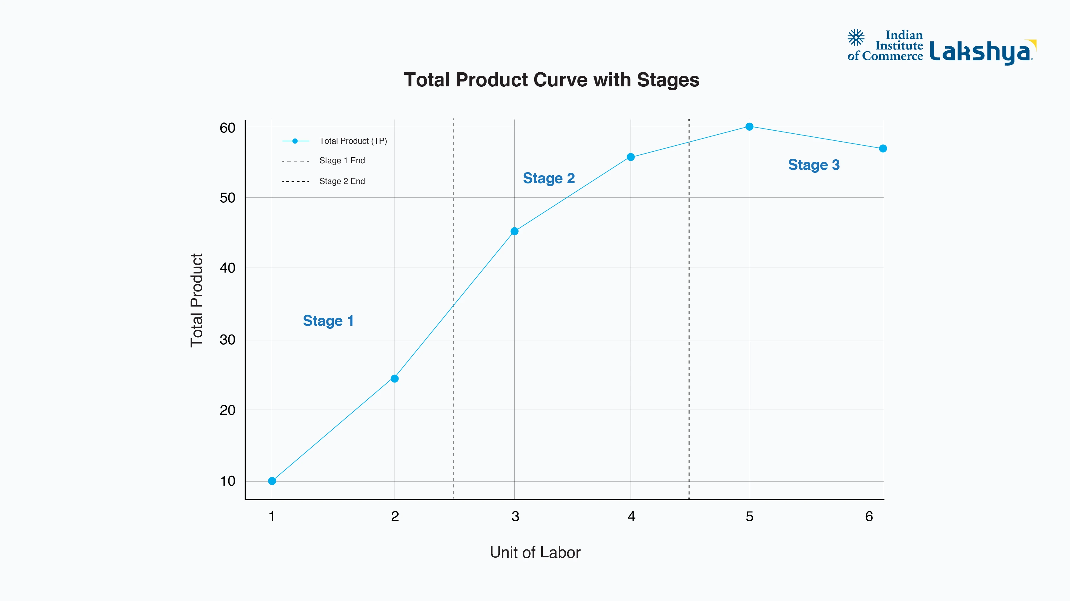
Total Product Curve with Stages:
 

• Stage 1 ends at around 2.5 units of labor.
• Stage 2 ends at around 4.5 units.
• Stage 3 begins after that, showing the decline in total product.
   

Here is a graphical representation of the Marginal and Average Product curve at different stages: 

 

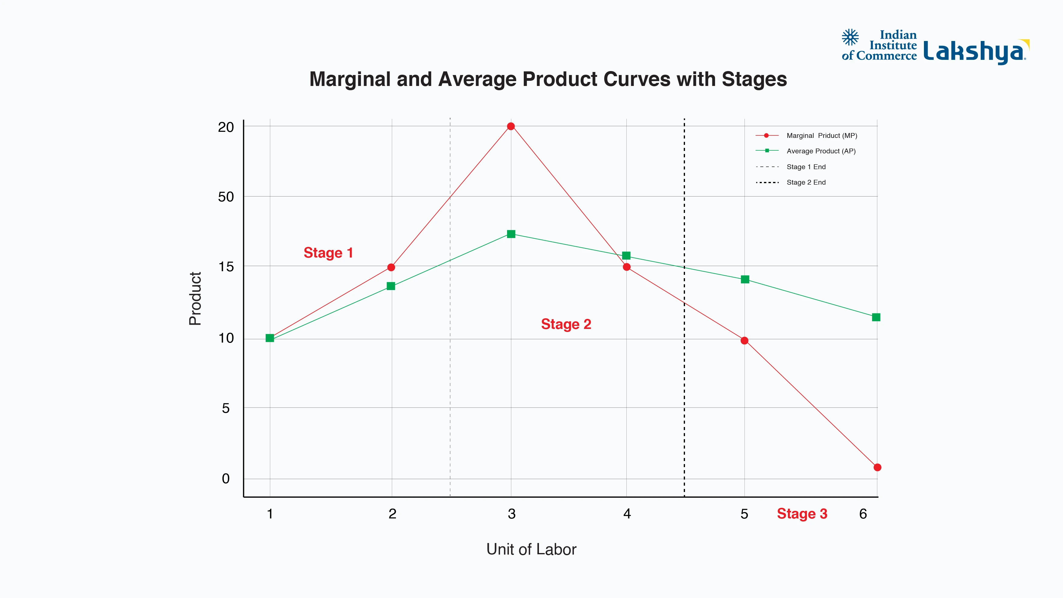
Marginal and Average Product Curves with Stages:
 

• The stages are similarly marked, with clear labels to show how marginal and average products behave across the different stages.
   

Conclusion

The Law of Variable Proportions is essential for businesses in managing production and maximizing efficiency. Understanding the stages of increasing, diminishing, and negative returns helps companies determine the optimal level of input use.

 

Want to understand how depreciation impacts production and economic decisions? Watch our detailed video now! 

 

 

 

Read More: 

• Negotiable Instruments Act 
• Trading and Profit & Loss Account
• Partnership Deed
• What are Equity Shares?

 

Keen on learning new topics about commerce every day, our Commerce Concepts for 11 & 12th students will give you a kickstart! 

 

Frequently Asked Questions (FAQs) 

What are the key takeaways from the law of variable proportions? 

The key takeaways from the law of variable proportions are: 

• Increasing returns 
• Diminishing returns 
• Negative returns 

How is the law of variable proportions significant in terms of economics?

The law of variable proportions helps businesses understand how to manage their resources effectively, the impact it will create on production, and determine the level of input needed for production efficiency. 

Is the law of variable proportions applicable in the long run? 

No, the law of variable proportions is not applicable in the long run because at least one fixed input determines the production output.